
AI For Trading:Project 7: Combine Signals for Enhanced Alpha (116)
Instructions
Each problem consists of a function to implement and instructions on how to implement the function. The parts of the function that need to be implemented are marked with a # TODO comment. After implementing the function, run the cell to test it against the unit tests we've provided. For each problem, we provide one or more unit tests from our project_tests package. These unit tests won't tell you if your answer is correct, but will warn you of any major errors. Your code will be checked for the correct solution when you submit it to Udacity.
Packages
When you implement the functions, you'll only need to you use the packages you've used in the classroom, like Pandas and Numpy. These packages will be imported for you. We recommend you don't add any import statements, otherwise the grader might not be able to run your code.
The other packages that we're importing are project_helper and project_tests. These are custom packages built to help you solve the problems. The project_helper module contains utility functions and graph functions. The project_tests contains the unit tests for all the problems.
Install Packages
import sys
!{sys.executable} -m pip install -r requirements.txt
...
Collecting alphalens==0.3.2 (from -r requirements.txt (line 1))
[?25l Downloading https://files.pythonhosted.org/packages/a5/dc/2f9cd107d0d4cf6223d37d81ddfbbdbf0d703d03669b83810fa6b97f32e5/alphalens-0.3.2.tar.gz (18.9MB)
[K 100% |████████████████████████████████| 18.9MB 1.7MB/s eta 0:00:01 7% 0 numpy-1.13.3 pandas-0.18.1 pandas-datareader-0.5.0 python-editor-1.0.4 requests-file-1.4.3 requests-ftp-0.3.1 scipy-1.0.0 sortedcontainers-2.1.0 tables-3.3.0 tqdm-4.19.5 zipline-1.2.0Load Packages
import project_helper
import project_tests

import numpy as np
import pandas as pd
from tqdm import tqdm
import matplotlib.pyplot as plt

%matplotlib inline
plt.style.use('ggplot')
plt.rcParams['figure.figsize'] = (14, 8)
Data Pipeline
Data Bundle
We'll be using Zipline to handle our data. We've created a end of day data bundle for this project. Run the cell below to register this data bundle in zipline.
import os
from zipline.data import bundles

os.environ['ZIPLINE_ROOT'] = os.path.join(os.getcwd(), '..', '..', 'data', 'project_7_eod')

ingest_func = bundles.csvdir.csvdir_equities(['daily'], project_helper.EOD_BUNDLE_NAME)
bundles.register(project_helper.EOD_BUNDLE_NAME, ingest_func)

print('Data Registered')
Data RegisteredBuild Pipeline Engine
We'll be using Zipline's pipeline package to access our data for this project. To use it, we must build a pipeline engine. Run the cell below to build the engine.
from zipline.pipeline import Pipeline
from zipline.pipeline.factors import AverageDollarVolume
from zipline.utils.calendars import get_calendar

universe = AverageDollarVolume(window_length=120).top(500)
trading_calendar = get_calendar('NYSE')
bundle_data = bundles.load(project_helper.EOD_BUNDLE_NAME)
engine = project_helper.build_pipeline_engine(bundle_data, trading_calendar)
View Data
With the pipeline engine built, let's get the stocks at the end of the period in the universe we're using.
universe_end_date = pd.Timestamp('2016-01-05', tz='UTC')

universe_tickers = engine\
    .run_pipeline(
        Pipeline(screen=universe),
        universe_end_date,
        universe_end_date)\
    .index.get_level_values(1)\
    .values.tolist()

universe_tickers[:5]
[Equity(0 [A]),
Equity(1 [AAL]),
Equity(2 [AAP]),
Equity(3 [AAPL]),
Equity(4 [ABBV])]Get Returns
Not that we have our pipeline built, let's access the returns data. We'll start by building a data portal.
from zipline.data.data_portal import DataPortal

data_portal = DataPortal(
    bundle_data.asset_finder,
    trading_calendar=trading_calendar,
    first_trading_day=bundle_data.equity_daily_bar_reader.first_trading_day,
    equity_minute_reader=None,
    equity_daily_reader=bundle_data.equity_daily_bar_reader,
    adjustment_reader=bundle_data.adjustment_reader)
To make the code easier to read, we've built the helper function get_pricing to get the pricing from the data portal.
def get_pricing(data_portal, trading_calendar, assets, start_date, end_date, field='close'):
    end_dt = pd.Timestamp(end_date.strftime('%Y-%m-%d'), tz='UTC', offset='C')
    start_dt = pd.Timestamp(start_date.strftime('%Y-%m-%d'), tz='UTC', offset='C')

    end_loc = trading_calendar.closes.index.get_loc(end_dt)
    start_loc = trading_calendar.closes.index.get_loc(start_dt)

    return data_portal.get_history_window(
        assets=assets,
        end_dt=end_dt,
        bar_count=end_loc - start_loc,
        frequency='1d',
        field=field,
        data_frequency='daily')
Alpha Factors
It's time to start working on the alpha factors. In this project, we'll use the following factors:
- Momentum 1 Year Factor
- Mean Reversion 5 Day Sector Neutral Smoothed Factor
- Overnight Sentiment Smoothed Factor
from zipline.pipeline.factors import CustomFactor, DailyReturns, Returns, SimpleMovingAverage, AnnualizedVolatility
from zipline.pipeline.data import USEquityPricing

factor_start_date = universe_end_date - pd.DateOffset(years=3, days=2)
sector = project_helper.Sector()

def momentum_1yr(window_length, universe, sector):
    return Returns(window_length=window_length, mask=universe) \
        .demean(groupby=sector) \
        .rank() \
        .zscore()

def mean_reversion_5day_sector_neutral_smoothed(window_length, universe, sector):
    unsmoothed_factor = -Returns(window_length=window_length, mask=universe) \
        .demean(groupby=sector) \
        .rank() \
        .zscore()
    return SimpleMovingAverage(inputs=[unsmoothed_factor], window_length=window_length) \
        .rank() \
        .zscore()

class CTO(Returns):
    """
    Computes the overnight return, per hypothesis from
    https://papers.ssrn.com/sol3/papers.cfm?abstract_id=2554010
    """
    inputs = [USEquityPricing.open, USEquityPricing.close]

    def compute(self, today, assets, out, opens, closes):
        """
        The opens and closes matrix is 2 rows x N assets, with the most recent at the bottom.
        As such, opens[-1] is the most recent open, and closes[0] is the earlier close
        """
        out[:] = (opens[-1] - closes[0]) / closes[0]

class TrailingOvernightReturns(Returns):
    """
    Sum of trailing 1m O/N returns
    """
    window_safe = True

    def compute(self, today, asset_ids, out, cto):
        out[:] = np.nansum(cto, axis=0)

def overnight_sentiment_smoothed(cto_window_length, trail_overnight_returns_window_length, universe):
    cto_out = CTO(mask=universe, window_length=cto_window_length)
    unsmoothed_factor = TrailingOvernightReturns(inputs=[cto_out], window_length=trail_overnight_returns_window_length) \
        .rank() \
        .zscore()
    return SimpleMovingAverage(inputs=[unsmoothed_factor], window_length=trail_overnight_returns_window_length) \
        .rank() \
        .zscore()
Combine the Factors to a single Pipeline
Let's add the factors to a pipeline.
universe = AverageDollarVolume(window_length=120).top(500)
sector = project_helper.Sector()

pipeline = Pipeline(screen=universe)
pipeline.add(
    momentum_1yr(252, universe, sector),
    'Momentum_1YR')
pipeline.add(
    mean_reversion_5day_sector_neutral_smoothed(20, universe, sector),
    'Mean_Reversion_Sector_Neutral_Smoothed')
pipeline.add(
    overnight_sentiment_smoothed(2, 10, universe),
    'Overnight_Sentiment_Smoothed')
Features and Labels
Let's create some features that we think will help the model make predictions.
"Universal" Quant Features
To capture the universe, we'll use the following as features:
- Stock Volatility 20d, 120d
- Stock Dollar Volume 20d, 120d
- Sector
pipeline.add(AnnualizedVolatility(window_length=20, mask=universe).rank().zscore(), 'volatility_20d')
pipeline.add(AnnualizedVolatility(window_length=120, mask=universe).rank().zscore(), 'volatility_120d')
pipeline.add(AverageDollarVolume(window_length=20, mask=universe).rank().zscore(), 'adv_20d')
pipeline.add(AverageDollarVolume(window_length=120, mask=universe).rank().zscore(), 'adv_120d')
pipeline.add(sector, 'sector_code')
Regime Features
We are going to try to capture market-wide regimes. To do that, we'll use the following features:
- High and low volatility 20d, 120d
- High and low dispersion 20d, 120d
class MarketDispersion(CustomFactor):
    inputs = [DailyReturns()]
    window_length = 1
    window_safe = True

    def compute(self, today, assets, out, returns):
        # returns are days in rows, assets across columns
        out[:] = np.sqrt(np.nanmean((returns - np.nanmean(returns))**2))

pipeline.add(SimpleMovingAverage(inputs=[MarketDispersion(mask=universe)], window_length=20), 'dispersion_20d')
pipeline.add(SimpleMovingAverage(inputs=[MarketDispersion(mask=universe)], window_length=120), 'dispersion_120d')
class MarketVolatility(CustomFactor):
inputs = [DailyReturns()]
window_length = 1
window_safe = True
def compute(self, today, assets, out, returns):
mkt_returns = np.nanmean(returns, axis=1)
out[:] = np.sqrt(260.* np.nanmean((mkt_returns-np.nanmean(mkt_returns))**2))
pipeline.add(MarketVolatility(window_length=20), 'market_vol_20d')
pipeline.add(MarketVolatility(window_length=120), 'market_vol_120d')Target
Let's try to predict the go forward 1-week return. When doing this, it's important to quantize the target. The factor we create is the trailing 5-day return.
pipeline.add(Returns(window_length=5, mask=universe).quantiles(2), 'return_5d')
pipeline.add(Returns(window_length=5, mask=universe).quantiles(25), 'return_5d_p')
Date Features
Let's make columns for the trees to split on that might capture trader/investor behavior due to calendar anomalies.
all_factors = engine.run_pipeline(pipeline, factor_start_date, universe_end_date)

all_factors['is_Janaury'] = all_factors.index.get_level_values(0).month == 1
all_factors['is_December'] = all_factors.index.get_level_values(0).month == 12
all_factors['weekday'] = all_factors.index.get_level_values(0).weekday
all_factors['quarter'] = all_factors.index.get_level_values(0).quarter
all_factors['qtr_yr'] = all_factors.quarter.astype('str') + '_' + all_factors.index.get_level_values(0).year.astype('str')
all_factors['month_end'] = all_factors.index.get_level_values(0).isin(pd.date_range(start=factor_start_date, end=universe_end_date, freq='BM'))
all_factors['month_start'] = all_factors.index.get_level_values(0).isin(pd.date_range(start=factor_start_date, end=universe_end_date, freq='BMS'))
all_factors['qtr_end'] = all_factors.index.get_level_values(0).isin(pd.date_range(start=factor_start_date, end=universe_end_date, freq='BQ'))
all_factors['qtr_start'] = all_factors.index.get_level_values(0).isin(pd.date_range(start=factor_start_date, end=universe_end_date, freq='BQS'))

all_factors.head()| Mean_Reversion_Sector_Neutral_Smoothed | Momentum_1YR | Overnight_Sentiment_Smoothed | adv_120d | adv_20d | dispersion_120d | dispersion_20d | market_vol_120d | market_vol_20d | return_5d | ... | volatility_20d | is_Janaury | is_December | weekday | quarter | qtr_yr | month_end | month_start | qtr_end | qtr_start | ||
|---|---|---|---|---|---|---|---|---|---|---|---|---|---|---|---|---|---|---|---|---|---|---|
| 2013-01-03 00:00:00+00:00 | Equity(0 [A]) | -0.26276899 | -1.20797813 | -1.48566901 | 1.33857307 | 1.39741144 | 0.01326964 | 0.01117804 | 0.12966421 | 0.13758558 | 0 | ... | -1.21980876 | True | False | 3 | 1 | 1_2013 | False | False | False | False |
5 rows × 23 columns
One Hot Encode Sectors
For the model to better understand the sector data, we'll one hot encode this data.
sector_lookup = pd.read_csv(
    os.path.join(os.getcwd(), '..', '..', 'data', 'project_7_sector', 'labels.csv'),
    index_col='Sector_i')['Sector'].to_dict()
sector_lookup

sector_columns = []
for sector_i, sector_name in sector_lookup.items():
    secotr_column = 'sector_{}'.format(sector_name)
    sector_columns.append(secotr_column)
    all_factors[secotr_column] = (all_factors['sector_code'] == sector_i)

all_factors[sector_columns].head()| sector_Healthcare | sector_Technology | sector_Consumer Defensive | sector_Industrials | sector_Utilities | sector_Financial Services | sector_Real Estate | sector_Communication Services | sector_Consumer Cyclical | sector_Energy | sector_Basic Materials | ||
|---|---|---|---|---|---|---|---|---|---|---|---|---|
| 2013-01-03 00:00:00+00:00 | Equity(0 [A]) | True | False | False | False | False | False | False | False | False | False | False |
| Equity(1 [AAL]) | False | False | False | True | False | False | False | False | False | False | False |
Shift Target
We'll use shifted 5 day returns for training the model.
all_factors['target'] = all_factors.groupby(level=1)['return_5d'].shift(-5)

all_factors[['return_5d','target']].reset_index().sort_values(['level_1', 'level_0']).head(10)| level_0 | level_1 | return_5d | target | |
|---|---|---|---|---|
| 0 | 2013-01-03 00:00:00+00:00 | Equity(0 [A]) | 0 | 0.00000000 |
| 471 | 2013-01-04 00:00:00+00:00 | Equity(0 [A]) | 0 | 0.00000000 |
| 942 | 2013-01-07 00:00:00+00:00 | Equity(0 [A]) | 0 | 0.00000000 |
| 1413 | 2013-01-08 00:00:00+00:00 | Equity(0 [A]) | 0 | 1.00000000 |
| 1884 | 2013-01-09 00:00:00+00:00 | Equity(0 [A]) | 0 | 0.00000000 |
| 2355 | 2013-01-10 00:00:00+00:00 | Equity(0 [A]) | 0 | 0.00000000 |
| 2826 | 2013-01-11 00:00:00+00:00 | Equity(0 [A]) | 0 | 0.00000000 |
| 3297 | 2013-01-14 00:00:00+00:00 | Equity(0 [A]) | 0 | 0.00000000 |
| 3768 | 2013-01-15 00:00:00+00:00 | Equity(0 [A]) | 1 | 0.00000000 |
| 4239 | 2013-01-16 00:00:00+00:00 | Equity(0 [A]) | 0 | 0.00000000 |
IID Check of Target
Let's see if the returns are independent and identically distributed.
from scipy.stats import spearmanr

def sp(group, col1_name, col2_name):
    x = group[col1_name]
    y = group[col2_name]
    return spearmanr(x, y)[0]

all_factors['target_p'] = all_factors.groupby(level=1)['return_5d_p'].shift(-5)
all_factors['target_1'] = all_factors.groupby(level=1)['return_5d'].shift(-4)
all_factors['target_2'] = all_factors.groupby(level=1)['return_5d'].shift(-3)
all_factors['target_3'] = all_factors.groupby(level=1)['return_5d'].shift(-2)
all_factors['target_4'] = all_factors.groupby(level=1)['return_5d'].shift(-1)

g = all_factors.dropna().groupby(level=0)
for i in range(4):
    label = 'target_'+str(i+1)
    ic = g.apply(sp, 'target', label)
    ic.plot(ylim=(-1, 1), label=label)
plt.legend(bbox_to_anchor=(1.04, 1), borderaxespad=0)
plt.title('Rolling Autocorrelation of Labels Shifted 1,2,3,4 Days')
plt.show()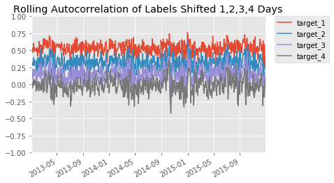
Question: What do you observe in the rolling autocorrelation of labels shifted?
#TODO: Put Answer In this Cell
Train/Valid/Test Splits
Now let's split the data into a train, validation, and test dataset. Implement the function train_valid_test_split to split the input samples, all_x, and targets values, all_y into a train, validation, and test dataset. The proportion sizes are train_size, valid_size, test_size respectively.
When splitting, make sure the data is in order from train, validation, and test respectivly. Say train_size is 0.7, valid_size is 0.2, and test_size is 0.1. The first 70 percent of all_x and all_y would be the train set. The next 20 percent of all_x and all_y would be the validation set. The last 10 percent of all_x and all_y would be the test set. Make sure not split a day between multiple datasets. It should be contained within a single dataset.
def train_valid_test_split(all_x, all_y, train_size, valid_size, test_size):
    """
    Generate the train, validation, and test dataset.

    Parameters
    ----------
    all_x : DataFrame
        All the input samples
    all_y : Pandas Series
        All the target values
    train_size : float
        The proportion of the data used for the training dataset
    valid_size : float
        The proportion of the data used for the validation dataset
    test_size : float
        The proportion of the data used for the test dataset

    Returns
    -------
    x_train : DataFrame
        The train input samples
    x_valid : DataFrame
        The validation input samples
    x_test : DataFrame
        The test input samples
    y_train : Pandas Series
        The train target values
    y_valid : Pandas Series
        The validation target values
    y_test : Pandas Series
        The test target values
    """
    assert train_size >= 0 and train_size <= 1.0
    assert valid_size >= 0 and valid_size <= 1.0
    assert test_size >= 0 and test_size <= 1.0
    assert train_size + valid_size + test_size == 1.0

    # TODO: Implement
    dates = all_x.index.levels[0]
    # print
    # print("all_x:\n", all_x)
    # print("dates:\n", dates)

    train_split = round(train_size*len(dates))
    valid_split = round(valid_size*len(dates)) + train_split
    test_split = round(test_size*len(dates)) + valid_split

    x_train = all_x.loc[:dates[train_split-1]]
    # print("x_train:\n", x_train)

    x_valid = all_x.loc[dates[train_split]:dates[valid_split-1]]
    x_test = all_x.loc[dates[valid_split]:]

    # 打印 all_y
    # print("all_y:\n", all_y)
    y_train = all_y.loc[:dates[train_split-1]]
    y_valid = all_y.loc[dates[train_split]:dates[valid_split-1]]
    y_test = all_y.loc[dates[valid_split]:]

    return x_train,x_valid,x_test,y_train,y_valid,y_test

project_tests.test_train_valid_test_split(train_valid_test_split)
Tests PassedWith train_valid_test_split implemented, let's split the data into a train, validation, and test set. For this, we'll use some of the features and the 5 day returns for our target.
features = [
    'Mean_Reversion_Sector_Neutral_Smoothed', 'Momentum_1YR',
    'Overnight_Sentiment_Smoothed', 'adv_120d', 'adv_20d',
    'dispersion_120d', 'dispersion_20d', 'market_vol_120d',
    'market_vol_20d', 'volatility_20d',
    'is_Janaury', 'is_December', 'weekday',
    'month_end', 'month_start', 'qtr_end', 'qtr_start'] + sector_columns
target_label = 'target'

temp = all_factors.dropna().copy()
X = temp[features]
y = temp[target_label]

X_train, X_valid, X_test, y_train, y_valid, y_test = train_valid_test_split(X, y, 0.6, 0.2, 0.2)

X_train.head()| Mean_Reversion_Sector_Neutral_Smoothed | Momentum_1YR | Overnight_Sentiment_Smoothed | adv_120d | adv_20d | dispersion_120d | dispersion_20d | market_vol_120d | market_vol_20d | volatility_20d | ... | sector_Technology | sector_Consumer Defensive | sector_Industrials | sector_Utilities | sector_Financial Services | sector_Real Estate | sector_Communication Services | sector_Consumer Cyclical | sector_Energy | sector_Basic Materials | ||
|---|---|---|---|---|---|---|---|---|---|---|---|---|---|---|---|---|---|---|---|---|---|---|
| 2013-01-03 00:00:00+00:00 | Equity(0 [A]) | -0.26276899 | -1.20797813 | -1.48566901 | 1.33857307 | 1.39741144 | 0.01326964 | 0.01117804 | 0.12966421 | 0.13758558 | -1.21980876 | ... | False | False | False | False | False | False | False | False | False | False |
5 rows × 28 columns
Random Forests
Visualize a Simple Tree
Let's see how a single tree would look using our data.
from IPython.display import display
from sklearn.tree import DecisionTreeClassifier

# This is to get consistent results between each run.
clf_random_state = 0

simple_clf = DecisionTreeClassifier(
    max_depth=3,
    criterion='entropy',
    random_state=clf_random_state)
simple_clf.fit(X_train, y_train)

display(project_helper.plot_tree_classifier(simple_clf, feature_names=features))
project_helper.rank_features_by_importance(simple_clf.feature_importances_, features)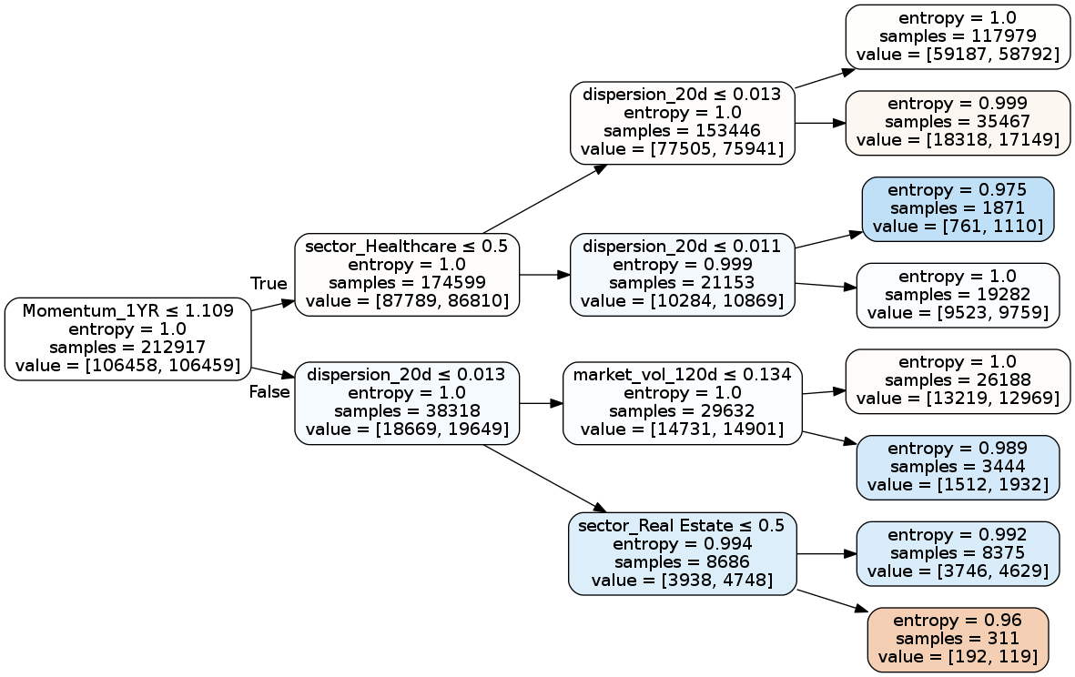
      Feature                                    Importance
 1. dispersion_20d                         (0.46843340608552875)
 2. market_vol_120d                        (0.19358730055081794)
 3. sector_Real Estate                     (0.12813661543951108)
 4. Momentum_1YR                           (0.11211962120010666)
 5. sector_Healthcare                      (0.09772305672403549)
 6. sector_Basic Materials                 (0.0)
 7. weekday                                (0.0)
 8. Overnight_Sentiment_Smoothed           (0.0)
 9. adv_120d                               (0.0)
10. adv_20d                                (0.0)
11. dispersion_120d                        (0.0)
12. market_vol_20d                         (0.0)
13. volatility_20d                         (0.0)
14. is_Janaury                             (0.0)
15. is_December                            (0.0)
16. month_end                              (0.0)
17. sector_Energy                          (0.0)
18. month_start                            (0.0)
19. qtr_end                                (0.0)
20. qtr_start                              (0.0)
21. sector_Technology                      (0.0)
22. sector_Consumer Defensive              (0.0)
23. sector_Industrials                     (0.0)
24. sector_Utilities                       (0.0)
25. sector_Financial Services              (0.0)
26. sector_Communication Services          (0.0)
27. sector_Consumer Cyclical               (0.0)
28. Mean_Reversion_Sector_Neutral_Smoothed (0.0)
Question: Why does dispersion_20d have the highest feature importance, when the first split is on the Momentum_1YR feature?
#TODO: Put Answer In this Cell
Train Random Forests with Different Tree Sizes
Let's build models using different tree sizes to find the model that best generalizes.
Parameters
When building the models, we'll use the following parameters.
n_days = 10
n_stocks = 500

clf_parameters = {
    'criterion': 'entropy',
    'min_samples_leaf': n_stocks * n_days,
    'oob_score': True,
    'n_jobs': -1,
    'random_state': clf_random_state}
n_trees_l = [50, 100, 250, 500, 1000]
Recall from the lesson, that we’ll choose a min_samples_leaf parameter to be small enough to allow the tree to fit the data with as much detail as possible, but not so much that it overfits. We can first propose 500, which is the number of assets in the estimation universe. Since we have about 500 stocks in the stock universe, we’ll want at least 500 stocks in a leaf for the leaf to make a prediction that is representative. It’s common to multiply this by 2,3,5 or 10, so we’d have min samples leaf of 500, 1000, 1500, 2500, and 5000. If we were to try these values, we’d notice that the model is “too good to be true” on the training data. A good rule of thumb for what is considered “too good to be true”, and therefore a sign of overfitting, is if the sharpe ratio is greater than 4. Based on this, we recommend using min_sampes_leaf of 10 * 500, or 5,000.
Feel free to try other values for these parameters, but also keep in mind that making too many small adjustments to hyper-parameters can lead to overfitting even the validation data, and therefore lead to less generalizable performance on the out-of-sample test set. So when trying different parameter values, choose values that are different enough in scale (i.e. 10, 20, 100 instead of 10,11,12).
from sklearn.ensemble import RandomForestClassifier

train_score = []
valid_score = []
oob_score = []
feature_importances = []

for n_trees in tqdm(n_trees_l, desc='Training Models', unit='Model'):
    clf = RandomForestClassifier(n_trees, **clf_parameters)
    clf.fit(X_train, y_train)

    train_score.append(clf.score(X_train, y_train.values))
    valid_score.append(clf.score(X_valid, y_valid.values))
    oob_score.append(clf.oob_score_)
    feature_importances.append(clf.feature_importances_)
Training Models: 100%|██████████| 5/5 [10:32<00:00, 126.52s/Model]Let's look at the accuracy of the classifiers over the number of trees.
project_helper.plot(
    [n_trees_l]*3,
    [train_score, valid_score, oob_score],
    ['train', 'validation', 'oob'],
    'Random Forrest Accuracy',
    'Number of Trees')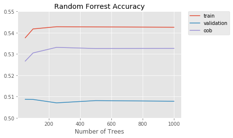
Question: 1) What do you observe with the accuracy vs tree size graph? 2) Does the graph indicate the model is overfitting or underfitting? Describe how it indicates this.
#TODO: Put Answer In this Cell
Now let's looks at the average feature importance of the classifiers.
print('Features Ranked by Average Importance:\n')
project_helper.rank_features_by_importance(np.average(feature_importances, axis=0), features)
Features Ranked by Average Importance:
Feature Importance
1. dispersion_20d (0.1269778070278301)
2. volatility_20d (0.12109751092486871)
3. market_vol_120d (0.10610349775271208)
4. market_vol_20d (0.1031284505504851)
5. Momentum_1YR (0.09619459615815973)
6. dispersion_120d (0.07964771723886842)
7. Overnight_Sentiment_Smoothed (0.07791967844615746)
8. Mean_Reversion_Sector_Neutral_Smoothed (0.06975870911774727)
9. adv_120d (0.05918153910377677)
10. adv_20d (0.05434312068691877)
11. sector_Healthcare (0.03158933275282147)
12. sector_Basic Materials (0.012648395225842244)
13. sector_Consumer Defensive (0.011217900024550611)
14. sector_Industrials (0.010608580029761724)
15. sector_Financial Services (0.009124102603531675)
16. weekday (0.008277277899941867)
17. sector_Real Estate (0.0058334489315844)
18. sector_Utilities (0.005173200127194804)
19. sector_Technology (0.004050360629711794)
20. sector_Consumer Cyclical (0.0038784870650338853)
21. sector_Energy (0.0026093313325679574)
22. is_Janaury (0.0004917284046585393)
23. is_December (0.00011882364724656508)
24. month_end (2.6404318028065363e-05)
25. qtr_end (0.0)
26. month_start (0.0)
27. qtr_start (0.0)
28. sector_Communication Services (0.0)You might notice that some of the features of low to no importance. We will be removing them when training the final model.
Model Results
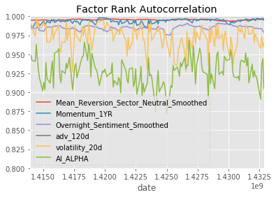
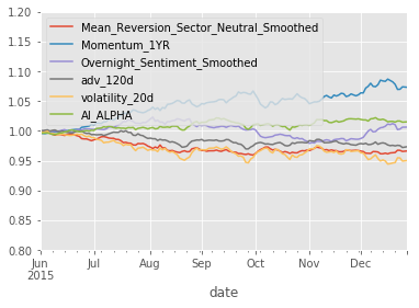
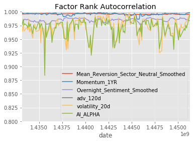
Let's look at some additional metrics to see how well a model performs. We've created the function show_sample_results to show the following results of a model:
- Sharpe Ratios
- Factor Returns
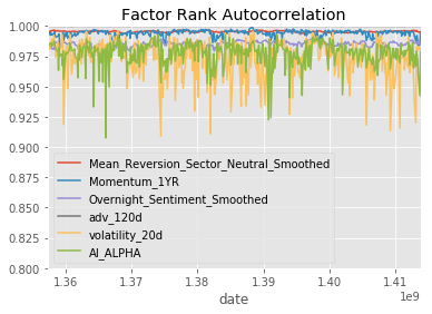
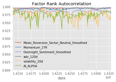
- Factor Rank Autocorrelation
import alphalens as al
all_assets = all_factors.index.levels[1].values.tolist()
all_pricing = get_pricing(
data_portal,
trading_calendar,
all_assets,
factor_start_date,
universe_end_date)
def show_sample_results(data, samples, classifier, factors, pricing=all_pricing):
# Calculate the Alpha Score
prob_array=[-1,1]
alpha_score = classifier.predict_proba(samples).dot(np.array(prob_array))
# Add Alpha Score to rest of the factors
alpha_score_label = 'AI_ALPHA'
factors_with_alpha = data.loc[samples.index].copy()
factors_with_alpha[alpha_score_label] = alpha_score
# Setup data for AlphaLens
print('Cleaning Data...\n')
factor_data = project_helper.build_factor_data(factors_with_alpha[factors + [alpha_score_label]], pricing)
print('\n-----------------------\n')
# Calculate Factor Returns and Sharpe Ratio
factor_returns = project_helper.get_factor_returns(factor_data)
sharpe_ratio = project_helper.sharpe_ratio(factor_returns)
# Show Results
print(' Sharpe Ratios')
print(sharpe_ratio.round(2))
project_helper.plot_factor_returns(factor_returns)
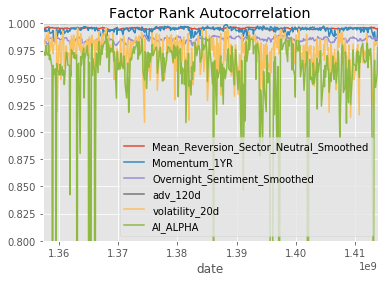
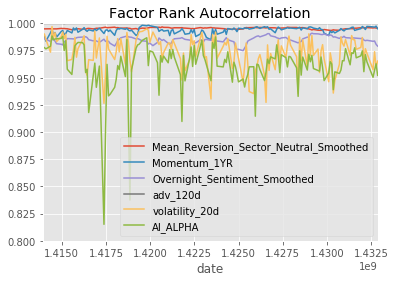
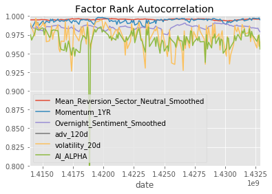
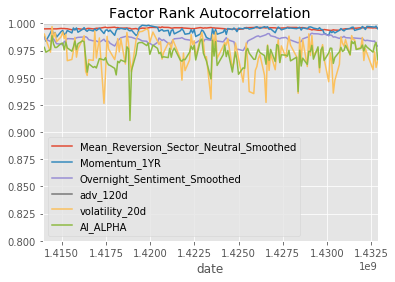
project_helper.plot_factor_rank_autocorrelation(factor_data)Results
Let's compare our AI Alpha factor to a few other factors. We'll use the following:
factor_names = [
    'Mean_Reversion_Sector_Neutral_Smoothed',
    'Momentum_1YR',
    'Overnight_Sentiment_Smoothed',
    'adv_120d',
    'volatility_20d']
Training Prediction
Let's see how well the model runs on training data.
show_sample_results(all_factors, X_train, clf, factor_names)Cleaning Data...
Dropped 0.2% entries from factor data: 0.2% in forward returns computation and 0.0% in binning phase (set max_loss=0 to see potentially suppressed Exceptions).
max_loss is 35.0%, not exceeded: OK!
Dropped 0.2% entries from factor data: 0.2% in forward returns computation and 0.0% in binning phase (set max_loss=0 to see potentially suppressed Exceptions).
max_loss is 35.0%, not exceeded: OK!
Dropped 0.2% entries from factor data: 0.2% in forward returns computation and 0.0% in binning phase (set max_loss=0 to see potentially suppressed Exceptions).
max_loss is 35.0%, not exceeded: OK!
Dropped 0.2% entries from factor data: 0.2% in forward returns computation and 0.0% in binning phase (set max_loss=0 to see potentially suppressed Exceptions).
max_loss is 35.0%, not exceeded: OK!
Dropped 0.2% entries from factor data: 0.2% in forward returns computation and 0.0% in binning phase (set max_loss=0 to see potentially suppressed Exceptions).
max_loss is 35.0%, not exceeded: OK!
Dropped 0.2% entries from factor data: 0.2% in forward returns computation and 0.0% in binning phase (set max_loss=0 to see potentially suppressed Exceptions).
max_loss is 35.0%, not exceeded: OK!
-----------------------
Sharpe Ratios
Mean_Reversion_Sector_Neutral_Smoothed 0.91000000
Momentum_1YR 0.19000000
Overnight_Sentiment_Smoothed 0.80000000
adv_120d 0.40000000
volatility_20d 1.06000000
AI_ALPHA 5.75000000
dtype: float64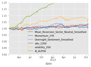
Validation Prediction
Let's see how well the model runs on validation data.
show_sample_results(all_factors, X_valid, clf, factor_names)Cleaning Data...
Dropped 0.0% entries from factor data: 0.0% in forward returns computation and 0.0% in binning phase (set max_loss=0 to see potentially suppressed Exceptions).
max_loss is 35.0%, not exceeded: OK!
Dropped 0.0% entries from factor data: 0.0% in forward returns computation and 0.0% in binning phase (set max_loss=0 to see potentially suppressed Exceptions).
...
max_loss is 35.0%, not exceeded: OK!
-----------------------
Sharpe Ratios
Mean_Reversion_Sector_Neutral_Smoothed 0.29000000
Momentum_1YR 0.76000000
Overnight_Sentiment_Smoothed -1.33000000
adv_120d -1.34000000
volatility_20d 0.09000000
AI_ALPHA 1.95000000
dtype: float64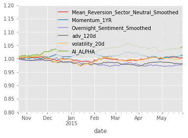
So that's pretty extraordinary. Even when the input factor returns are sideways to down, the AI Alpha is positive with Sharpe Ratio > 2. If we hope that this model will perform well in production we need to correct though for the non-IID labels and mitigate likely overfitting.
Overlapping Samples
Let's fix this by removing overlapping samples. We can do a number of things:
- Don't use overlapping samples
- Use BaggingClassifier's
max_samples - Build an ensemble of non-overlapping trees
In this project, we'll do all three methods and compare.
Drop Overlapping Samples
This is the simplest of the three methods. We'll just drop any overlapping samples from the dataset. Implement the non_overlapping_samples function to return a new dataset overlapping samples.
def non_overlapping_samples(x, y, n_skip_samples, start_i=0):
    """
    Get the non overlapping samples.

    Parameters
    ----------
    x : DataFrame
        The input samples
    y : Pandas Series
        The target values
    n_skip_samples : int
        The number of samples to skip
    start_i : int
        The starting index to use for the data

    Returns
    -------
    non_overlapping_x : 2 dimensional Ndarray
        The non overlapping input samples
    non_overlapping_y : 1 dimensional Ndarray
        The non overlapping target values
    """
    assert len(x.shape) == 2
    assert len(y.shape) == 1

    # TODO: Implement
    non_overlapping_x = x.loc[x.index.levels[0][start_i::n_skip_samples+1].tolist()]
    non_overlapping_y = y.loc[y.index.levels[0][start_i::n_skip_samples+1].tolist()]
    return non_overlapping_x,non_overlapping_y

project_tests.test_non_overlapping_samples(non_overlapping_samples)
Tests PassedWith the dataset created without overlapping samples, lets train a new model and look at the results.
Train Model
train_score = []
valid_score = []
oob_score = []

for n_trees in tqdm(n_trees_l, desc='Training Models', unit='Model'):
    clf = RandomForestClassifier(n_trees, **clf_parameters)
    clf.fit(*non_overlapping_samples(X_train, y_train, 4))

    train_score.append(clf.score(X_train, y_train.values))
    valid_score.append(clf.score(X_valid, y_valid.values))
    oob_score.append(clf.oob_score_)
Training Models: 100%|██████████| 5/5 [01:11<00:00, 14.22s/Model]Results
project_helper.plot(
    [n_trees_l]*3,
    [train_score, valid_score, oob_score],
    ['train', 'validation', 'oob'],
    'Random Forrest Accuracy',
    'Number of Trees')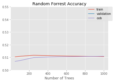
show_sample_results(all_factors, X_valid, clf, factor_names)Cleaning Data...
Dropped 0.0% entries from factor data: 0.0% in forward returns computation and 0.0% in binning phase (set max_loss=0 to see potentially suppressed Exceptions).
max_loss is 35.0%, not exceeded: OK!
...
Dropped 0.0% entries from factor data: 0.0% in forward returns computation and 0.0% in binning phase (set max_loss=0 to see potentially suppressed Exceptions).
max_loss is 35.0%, not exceeded: OK!
-----------------------
Sharpe Ratios
Mean_Reversion_Sector_Neutral_Smoothed 0.29000000
Momentum_1YR 0.76000000
Overnight_Sentiment_Smoothed -1.33000000
adv_120d -1.34000000
volatility_20d 0.09000000
AI_ALPHA -0.37000000
dtype: float64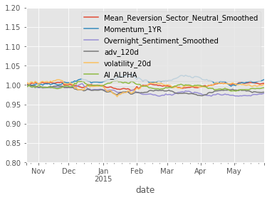
This looks better, but we are throwing away a lot of information by taking every 5th row.
Use BaggingClassifier's max_samples
In this method, we'll set max_samples to be on the order of the average uniqueness of the labels. Since RandomForrestClassifier does not take this param, we're using BaggingClassifier. Implement bagging_classifier to build the bagging classifier.
from sklearn.ensemble import BaggingClassifier
from sklearn.tree import DecisionTreeClassifier

def bagging_classifier(n_estimators, max_samples, max_features, parameters):
    """
    Build the bagging classifier.

    Parameters
    ----------
    n_estimators : int
        The number of base estimators in the ensemble
    max_samples : float
        The proportion of input samples drawn from when training each base estimator
    max_features : float
        The proportion of input sample features drawn from when training each base estimator
    parameters : dict
        Parameters to use in building the bagging classifier
        It should contain the following parameters:
            criterion
            min_samples_leaf
            oob_score
            n_jobs
            random_state

    Returns
    -------
    bagging_clf : Scikit-Learn BaggingClassifier
        The bagging classifier
    """

    required_parameters = {'criterion', 'min_samples_leaf', 'oob_score', 'n_jobs', 'random_state'}
    assert not required_parameters - set(parameters.keys())

    # TODO: Implement
    bagging_clf = BaggingClassifier(base_estimator=DecisionTreeClassifier(criterion=parameters['criterion'],min_samples_leaf= parameters['min_samples_leaf']),\
                                    n_estimators=n_estimators, \
                                    max_samples=max_samples, \
                                    max_features=max_features,\
                                    oob_score = parameters['oob_score'],\
                                    n_jobs = parameters['n_jobs'],\
                                    random_state = parameters['random_state']
                                   )

    return bagging_clf

project_tests.test_bagging_classifier(bagging_classifier)
Tests PassedWith the bagging classifier built, lets train a new model and look at the results.
Train Model
train_score = []
valid_score = []
oob_score = []

for n_trees in tqdm(n_trees_l, desc='Training Models', unit='Model'):
    clf = bagging_classifier(n_trees, 0.2, 1.0, clf_parameters)
    clf.fit(X_train, y_train)

    train_score.append(clf.score(X_train, y_train.values))
    valid_score.append(clf.score(X_valid, y_valid.values))
    oob_score.append(clf.oob_score_)
Training Models: 100%|██████████| 5/5 [18:01<00:00, 216.30s/Model]Results
project_helper.plot(
    [n_trees_l]*3,
    [train_score, valid_score, oob_score],
    ['train', 'validation', 'oob'],
    'Random Forrest Accuracy',
    'Number of Trees')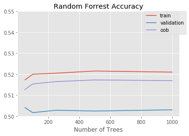
show_sample_results(all_factors, X_valid, clf, factor_names)Cleaning Data...
Dropped 0.0% entries from factor data: 0.0% in forward returns computation and 0.0% in binning phase (set max_loss=0 to see potentially suppressed Exceptions).
max_loss is 35.0%, not exceeded: OK!
...
Dropped 0.0% entries from factor data: 0.0% in forward returns computation and 0.0% in binning phase (set max_loss=0 to see potentially suppressed Exceptions).
max_loss is 35.0%, not exceeded: OK!
-----------------------
Sharpe Ratios
Mean_Reversion_Sector_Neutral_Smoothed 0.29000000
Momentum_1YR 0.76000000
Overnight_Sentiment_Smoothed -1.33000000
adv_120d -1.34000000
volatility_20d 0.09000000
AI_ALPHA 0.78000000
dtype: float64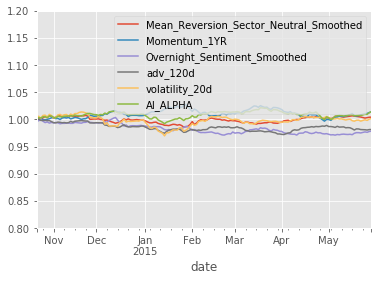
This seems much "better" in the sense that we have much better fidelity between the three.
Build an ensemble of non-overlapping trees
The last method is to create ensemble of non-overlapping trees. Here we are going to write a custom scikit-learn estimator. We inherit from VotingClassifier and we override the fit method so we fit on non-overlapping periods.
import abc

from sklearn.ensemble import VotingClassifier
from sklearn.base import clone
from sklearn.preprocessing import LabelEncoder
from sklearn.utils import Bunch

class NoOverlapVoterAbstract(VotingClassifier):
    @abc.abstractmethod
    def _calculate_oob_score(self, classifiers):
        raise NotImplementedError

    @abc.abstractmethod
    def _non_overlapping_estimators(self, x, y, classifiers, n_skip_samples):
        raise NotImplementedError

    def __init__(self, estimator, voting='soft', n_skip_samples=4):
        # List of estimators for all the subsets of data
        estimators = [('clf'+str(i), estimator) for i in range(n_skip_samples + 1)]

        self.n_skip_samples = n_skip_samples
        super().__init__(estimators, voting)

    def fit(self, X, y, sample_weight=None):
        estimator_names, clfs = zip(*self.estimators)
        self.le_ = LabelEncoder().fit(y)
        self.classes_ = self.le_.classes_

        clone_clfs = [clone(clf) for clf in clfs]
        self.estimators_ = self._non_overlapping_estimators(X, y, clone_clfs, self.n_skip_samples)
        self.named_estimators_ = Bunch(**dict(zip(estimator_names, self.estimators_)))
        self.oob_score_ = self._calculate_oob_score(self.estimators_)

        return self
You might notice that two of the functions are abstracted. These will be the functions that you need to implement.
OOB Score
In order to get the correct OOB score, we need to take the average of all the estimator's OOB scores. Implement calculate_oob_score to calculate this score.
def calculate_oob_score(classifiers):
    """
    Calculate the mean out-of-bag score from the classifiers.

    Parameters
    ----------
    classifiers : list of Scikit-Learn Classifiers
        The classifiers used to calculate the mean out-of-bag score

    Returns
    -------
    oob_score : float
        The mean out-of-bag score
    """

    # TODO: Implement

    return np.mean([o.oob_score_ for o in classifiers])

project_tests.test_calculate_oob_score(calculate_oob_score)
Tests PassedNon Overlapping Estimators
With calculate_oob_score implemented, let's create non overlapping estimators. Implement non_overlapping_estimators to build non overlapping subsets of the data, then run a estimator on each subset of data.
def non_overlapping_estimators(x, y, classifiers, n_skip_samples):
    """
    Fit the classifiers to non overlapping data.

    Parameters
    ----------
    x : DataFrame
        The input samples
    y : Pandas Series
        The target values
    classifiers : list of Scikit-Learn Classifiers
        The classifiers used to fit on the non overlapping data
    n_skip_samples : int
        The number of samples to skip

    Returns
    -------
    fit_classifiers : list of Scikit-Learn Classifiers
        The classifiers fit to the the non overlapping data
    """

    # TODO: Implement
    fit_classifiers=[]
    for i in range(len(classifiers)):
            non_overlapping_x ,non_overlapping_y = non_overlapping_samples(x, y, n_skip_samples, start_i=i)
            fit_classifiers.append( classifiers[i].fit(non_overlapping_x,non_overlapping_y))

    return fit_classifiers

project_tests.test_non_overlapping_estimators(non_overlapping_estimators)
Tests Passedclass NoOverlapVoter(NoOverlapVoterAbstract):
def _calculate_oob_score(self, classifiers):
return calculate_oob_score(classifiers)
def _non_overlapping_estimators(self, x, y, classifiers, n_skip_samples):
return non_overlapping_estimators(x, y, classifiers, n_skip_samples)Now that we have our NoOverlapVoter class, let's train it.
Train Model
train_score = []
valid_score = []
oob_score = []

for n_trees in tqdm(n_trees_l, desc='Training Models', unit='Model'):
    clf = RandomForestClassifier(n_trees, **clf_parameters)

    clf_nov = NoOverlapVoter(clf)
    clf_nov.fit(X_train, y_train)

    train_score.append(clf_nov.score(X_train, y_train.values))
    valid_score.append(clf_nov.score(X_valid, y_valid.values))
    oob_score.append(clf_nov.oob_score_)
Training Models: 100%|██████████| 5/5 [05:56<00:00, 71.36s/Model]Results
project_helper.plot(
    [n_trees_l]*3,
    [train_score, valid_score, oob_score],
    ['train', 'validation', 'oob'],
    'Random Forrest Accuracy',
    'Number of Trees')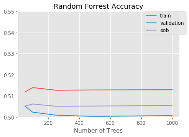
show_sample_results(all_factors, X_valid, clf_nov, factor_names)Cleaning Data...
Dropped 0.0% entries from factor data: 0.0% in forward returns computation and 0.0% in binning phase (set max_loss=0 to see potentially suppressed Exceptions).
...
Dropped 0.0% entries from factor data: 0.0% in forward returns computation and 0.0% in binning phase (set max_loss=0 to see potentially suppressed Exceptions).
max_loss is 35.0%, not exceeded: OK!
-----------------------
Sharpe Ratios
Mean_Reversion_Sector_Neutral_Smoothed 0.29000000
Momentum_1YR 0.76000000
Overnight_Sentiment_Smoothed -1.33000000
adv_120d -1.34000000
volatility_20d 0.09000000
AI_ALPHA 0.29000000
dtype: float64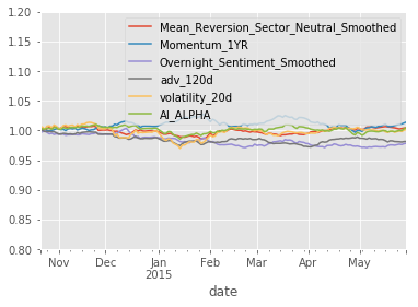
Final Model
Re-Training Model
In production, we would roll forward the training. Typically you would re-train up to the "current day" and then test. Here, we will train on the train & validation dataset.
n_trees = 500

clf = RandomForestClassifier(n_trees, **clf_parameters)
clf_nov = NoOverlapVoter(clf)
clf_nov.fit(
    pd.concat([X_train, X_valid]),
    pd.concat([y_train, y_valid]))
NoOverlapVoter(estimator=None, n_skip_samples=4, voting='soft')Results
Accuracy
print('train: {}, oob: {}, valid: {}'.format(
    clf_nov.score(X_train, y_train.values),
    clf_nov.score(X_valid, y_valid.values),
    clf_nov.oob_score_))
train: 0.5139232658735564, oob: 0.5122386644165191, valid: 0.5068127879069977Train
show_sample_results(all_factors, X_train, clf_nov, factor_names)Cleaning Data...
Dropped 0.2% entries from factor data: 0.2% in forward returns computation and 0.0% in binning phase (set max_loss=0 to see potentially suppressed Exceptions).
max_loss is 35.0%, not exceeded: OK!
...
Dropped 0.2% entries from factor data: 0.2% in forward returns computation and 0.0% in binning phase (set max_loss=0 to see potentially suppressed Exceptions).
max_loss is 35.0%, not exceeded: OK!
-----------------------
Sharpe Ratios
Mean_Reversion_Sector_Neutral_Smoothed 0.91000000
Momentum_1YR 0.19000000
Overnight_Sentiment_Smoothed 0.80000000
adv_120d 0.40000000
volatility_20d 1.06000000
AI_ALPHA 2.32000000
dtype: float64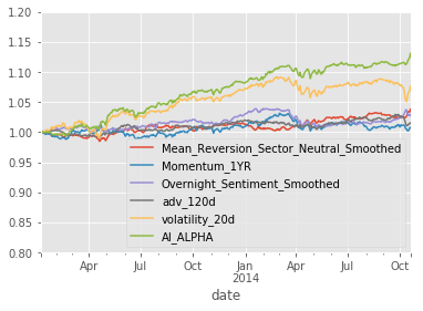
Validation
show_sample_results(all_factors, X_valid, clf_nov, factor_names)Cleaning Data...
Dropped 0.0% entries from factor data: 0.0% in forward returns computation and 0.0% in binning phase (set max_loss=0 to see potentially suppressed Exceptions).
max_loss is 35.0%, not exceeded: OK!
...
Dropped 0.0% entries from factor data: 0.0% in forward returns computation and 0.0% in binning phase (set max_loss=0 to see potentially suppressed Exceptions).
max_loss is 35.0%, not exceeded: OK!
-----------------------
Sharpe Ratios
Mean_Reversion_Sector_Neutral_Smoothed 0.29000000
Momentum_1YR 0.76000000
Overnight_Sentiment_Smoothed -1.33000000
adv_120d -1.34000000
volatility_20d 0.09000000
AI_ALPHA 2.89000000
dtype: float64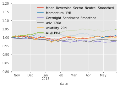
Test
show_sample_results(all_factors, X_test, clf_nov, factor_names)Cleaning Data...
Dropped 0.0% entries from factor data: 0.0% in forward returns computation and 0.0% in binning phase (set max_loss=0 to see potentially suppressed Exceptions).
max_loss is 35.0%, not exceeded: OK!
-----------------------
Sharpe Ratios
Mean_Reversion_Sector_Neutral_Smoothed -2.01000000
Momentum_1YR 2.60000000
Overnight_Sentiment_Smoothed 0.33000000
adv_120d -1.57000000
volatility_20d -1.68000000
AI_ALPHA 0.90000000
dtype: float64
...
So, hopefully you are appropriately amazed by this. Despite the significant differences between the factor performances in the three sets, the AI APLHA is able to deliver positive performance.
为者常成,行者常至
自由转载-非商用-非衍生-保持署名(创意共享3.0许可证)


