
AI For Trading:Overfitting Exercise (119)
Overfitting Exercise
In this exercise, we'll build a model that, as you'll see, dramatically overfits the training data. This will allow you to see what overfitting can "look like" in practice.
import os
import pandas as pd
import numpy as np
import math
import matplotlib.pyplot as plt
For this exercise, we'll use gradient boosted trees. In order to implement this model, we'll use the XGBoost package.
! pip install xgboostRequirement already satisfied: xgboost in /opt/conda/lib/python3.6/site-packages (0.90)
Requirement already satisfied: scipy in /opt/conda/lib/python3.6/site-packages (from xgboost) (0.19.1)
Requirement already satisfied: numpy in /opt/conda/lib/python3.6/site-packages (from xgboost) (1.12.1)import xgboost as xgbHere, we define a few helper functions.
# number of rows in a dataframe
def nrow(df):
    return(len(df.index))

# number of columns in a dataframe
def ncol(df):
    return(len(df.columns))

# flatten nested lists/arrays
flatten = lambda l: [item for sublist in l for item in sublist]

# combine multiple arrays into a single list
def c(*args):
    return(flatten([item for item in args]))
In this exercise, we're going to try to predict the returns of the S&P 500 ETF. This may be a futile endeavor, since many experts consider the S&P 500 to be essentially unpredictable, but it will serve well for the purpose of this exercise. The following cell loads the data.
df = pd.read_csv("SPYZ.csv")As you can see, the data file has four columns, Date, Close, Volume and Return.
df.head()| Date | Close | Volume | Return | |
|---|---|---|---|---|
| 0 | 1999-12-31 | 146.8750 | 3172700 | 0.001598 |
| 1 | 2000-01-03 | 145.4375 | 8164300 | -0.009787 |
| 2 | 2000-01-04 | 139.7500 | 8089800 | -0.039106 |
| 3 | 2000-01-05 | 140.0000 | 12177900 | 0.001789 |
| 4 | 2000-01-06 | 137.7500 | 6227200 | -0.016071 |
n = nrow(df)Next, we'll form our predictors/features. In the cells below, we create four types of features. We also use a parameter, K, to set the number of each type of feature to build. With a K of 25, 100 features will be created. This should already seem like a lot of features, and alert you to the potential that the model will be overfit.
predictors = []

# we'll create a new DataFrame to hold the data that we'll use to train the model
# we'll create it from the `Return` column in the original DataFrame, but rename that column `y`
model_df = pd.DataFrame(data = df['Return']).rename(columns = {"Return" : "y"})

# IMPORTANT: this sets how many of each of the following four predictors to create
K = 25
Now, you write the code to create the four types of predictors.
for L in range(1,K+1):
    # this predictor is just the return L days ago, where L goes from 1 to K
    # these predictors will be named `R1`, `R2`, etc.
    pR = "".join(["R",str(L)])
    predictors.append(pR)
    for i in range(K+1,n):
        # TODO: fill in the code to assign the return from L days before to the ith row of this predictor in `model_df`
        model_df.loc[i, pR] = df.loc[i-L, 'Return']

    # this predictor is the return L days ago, squared, where L goes from 1 to K
    # these predictors will be named `Rsq1`, `Rsq2`, etc.
    pR2 = "".join(["Rsq",str(L)])
    predictors.append(pR2)
    for i in range(K+1,n):
        # TODO: fill in the code to assign the squared return from L days before to the ith row of this predictor
        # in `model_df`
        model_df.loc[i, pR2] = (df.loc[i-L, 'Return']) ** 2

    # this predictor is the log volume L days ago, where L goes from 1 to K
    # these predictors will be named `V1`, `V2`, etc.
    pV = "".join(["V",str(L)])
    predictors.append(pV)
    for i in range(K+1,n):
        # TODO: fill in the code to assign the log of the volume from L days before to the ith row of this predictor
        # in `model_df`
        # Add 1 to the volume before taking the log
        model_df.loc[i, pV] = math.log(1.0 + df.loc[i-L, 'Volume'])

    # this predictor is the product of the return and the log volume from L days ago, where L goes from 1 to K
    # these predictors will be named `RV1`, `RV2`, etc.
    pRV = "".join(["RV",str(L)])
    predictors.append(pRV)
    for i in range(K+1,n):
        # TODO: fill in the code to assign the product of the return and the log volume from L days before to the
        # ith row of this predictor in `model_df`
        model_df.loc[i, pRV] = model_df.loc[i,pR] * model_df.loc[i, pV]
Let's take a look at the predictors we've created.
model_df.iloc[100:105,:]| y | R1 | Rsq1 | V1 | RV1 | R2 | Rsq2 | V2 | RV2 | R3 | ... | V23 | RV23 | R24 | Rsq24 | V24 | RV24 | R25 | Rsq25 | V25 | RV25 | |
|---|---|---|---|---|---|---|---|---|---|---|---|---|---|---|---|---|---|---|---|---|---|
| 100 | 0.016304 | -0.014726 | 0.000217 | 15.892349 | -0.234024 | -0.007529 | 0.000057 | 16.198698 | -0.121956 | -0.018688 | ... | 15.959991 | 0.076664 | -0.009302 | 0.000087 | 15.695540 | -0.145995 | 0.026421 | 0.000698 | 16.209371 | 0.428273 |
| 101 | -0.017157 | 0.016304 | 0.000266 | 16.221058 | 0.264474 | -0.014726 | 0.000217 | 15.892349 | -0.234024 | -0.007529 | ... | 16.372203 | -0.177882 | 0.004804 | 0.000023 | 15.959991 | 0.076664 | -0.009302 | 0.000087 | 15.695540 | -0.145995 |
| 102 | 0.001133 | -0.017157 | 0.000294 | 15.929221 | -0.273290 | 0.016304 | 0.000266 | 16.221058 | 0.264474 | -0.014726 | ... | 16.461827 | 0.683503 | -0.010865 | 0.000118 | 16.372203 | -0.177882 | 0.004804 | 0.000023 | 15.959991 | 0.076664 |
| 104 | 0.000657 | 0.034194 | 0.001169 | 15.494960 | 0.529838 | 0.001133 | 0.000001 | 15.387039 | 0.017437 | -0.017157 | ... | 16.562480 | -0.054770 | -0.011285 | 0.000127 | 15.858172 | -0.178954 | 0.041520 | 0.001724 | 16.461827 | 0.683503 |
Next, we create a DataFrame that holds the recent volatility of the ETF's returns, as measured by the standard deviation of a sliding window of the past 20 days' returns.
vol_df = pd.DataFrame(data = df[['Return']])

for i in range(K+1,n):
    # TODO: create the code to assign the standard deviation of the return from the time period starting
    # 20 days before day i, up to the day before day i, to the ith row of `vol_df`
    vol_df.loc[i, 'vol'] = np.std(vol_df.loc[(i-20):(i-1), 'Return'])
Let's take a quick look at the result.
vol_df.iloc[100:105,:]| Return | vol | |
|---|---|---|
| 100 | 0.016304 | 0.013069 |
| 101 | -0.017157 | 0.013615 |
| 102 | 0.001133 | 0.014007 |
| 103 | 0.034194 | 0.014008 |
| 104 | 0.000657 | 0.015792 |
Now that we have our data, we can start thinking about training a model.
# for training, we'll use all the data except for the first K days, for which the predictors' values are NaNs
model = model_df.iloc[K:n,:]
In the cell below, first split the data into train and test sets, and then split off the targets from the predictors.
# Split data into train and test sets
train_size = 2.0/3.0
breakpoint = round(nrow(model) * train_size)

# TODO: fill in the code to split off the chunk of data up to the breakpoint as the training set, and
# assign the rest as the test set.
training_data = model.iloc[1:breakpoint,:]
print(training_data.head(5))

test_data = model.loc[breakpoint : nrow(model),]

# TODO: Split training data and test data into targets (Y) and predictors (X), for the training set and the test set
X_train = training_data.iloc[:,1:ncol(training_data)]
Y_train = training_data.iloc[:,0]
X_test = test_data.iloc[:, 1:ncol(training_data)]
Y_test = test_data.iloc[:,0]
y R1 Rsq1 V1 RV1 R2 Rsq2 \
26 0.013608 -0.001534 0.000002 15.581234 -0.023908 -0.004146 0.000017
27 -0.021004 0.013608 0.000185 15.412167 0.209736 -0.001534 0.000002
28 0.001990 -0.021004 0.000441 15.956929 -0.335166 0.013608 0.000185
29 -0.020309 0.001990 0.000004 15.716214 0.031282 -0.021004 0.000441
30 0.005859 -0.020309 0.000412 16.102901 -0.327034 0.001990 0.000004
V2 RV2 R3 ... V23 RV23 R24 \
26 15.409916 -0.063895 0.015064 ... 16.315133 0.029185 -0.039106
27 15.581234 -0.023908 -0.004146 ... 15.644438 -0.251429 0.001789
28 15.412167 0.209736 -0.001534 ... 15.903243 0.923601 -0.016071
29 15.956929 -0.335166 0.013608 ... 15.563249 0.053390 0.058076
30 15.716214 0.031282 -0.021004 ... 15.821534 -0.209601 0.003430
Rsq24 V24 RV24 R25 Rsq25 V25 RV25
26 0.001529 15.906115 -0.622027 -0.009787 0.000096 15.915282 -0.155767
27 0.000003 16.315133 0.029185 -0.039106 0.001529 15.906115 -0.622027
28 0.000258 15.644438 -0.251429 0.001789 0.000003 16.315133 0.029185
29 0.003373 15.903243 0.923601 -0.016071 0.000258 15.644438 -0.251429
30 0.000012 15.563249 0.053390 0.058076 0.003373 15.903243 0.923601
[5 rows x 101 columns]Great, now that we have our data, let's train the model.
# DMatrix is a internal data structure that used by XGBoost which is optimized for both memory efficiency
# and training speed.
dtrain = xgb.DMatrix(X_train, Y_train)

# Train the XGBoost model
param = { 'max_depth':20, 'silent':1 }
num_round = 20
xgModel = xgb.train(param, dtrain, num_round)
/opt/conda/lib/python3.6/site-packages/xgboost/core.py:587: FutureWarning: Series.base is deprecated and will be removed in a future version
if getattr(data, 'base', None) is not None and \
/opt/conda/lib/python3.6/site-packages/xgboost/core.py:588: FutureWarning: Series.base is deprecated and will be removed in a future version
data.base is not None and isinstance(data, np.ndarray) \Now let's predict the returns for the S&P 500 ETF in both the train and test periods. If the model is successful, what should the train and test accuracies look like? What would be a key sign that the model has overfit the training data?
Todo: Before you run the next cell, write down what you expect to see if the model is overfit.
# Make the predictions on the test data
preds_train = xgModel.predict(xgb.DMatrix(X_train))
preds_test = xgModel.predict(xgb.DMatrix(X_test))
Let's quickly look at the mean squared error of the predictions on the training and testing sets.
# TODO: Calculate the mean squared error on the training set
msetrain = sum((preds_train-Y_train)**2)/len(preds_train)
msetrain
Exception ignored in: <bound method Booster.__del__ of <xgboost.core.Booster object at 0x7f6da6e7d780>>
Traceback (most recent call last):
File "/opt/conda/lib/python3.6/site-packages/xgboost/core.py", line 957, in __del__
if self.handle is not None:
AttributeError: 'Booster' object has no attribute 'handle'
1.6237099209080407e-06# TODO: Calculate the mean squared error on the test set
msetest = sum((preds_test-Y_test)**2)/len(preds_test)
msetest7.711855498216044e-05Looks like the mean squared error on the test set is an order of magnitude greater than on the training set. Not a good sign. Now let's do some quick calculations to gauge how this would translate into performance.
# combine prediction arrays into a single list
predictions = c(preds_train, preds_test)
responses = c(Y_train, Y_test)

# as a holding size, we'll take predicted return divided by return variance
# this is mean-variance optimization with a single asset
vols = vol_df.loc[K:n,'vol']
position_size = predictions / vols ** 2

# TODO: Calculate pnl. Pnl in each time period is holding * realized return.
performance = position_size * responses

# plot simulated performance
plt.plot(np.cumsum(performance))
plt.ylabel('Simulated Performance')
plt.axvline(x=breakpoint, c = 'r')
plt.show()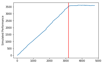
Our simulated returns accumulate throughout the training period, but they are absolutely flat in the testing period. The model has no predictive power whatsoever in the out-of-sample period.
Can you think of a few reasons our simulation of performance is unrealistic?
# TODO: Answer the above question.为者常成,行者常至
自由转载-非商用-非衍生-保持署名(创意共享3.0许可证)


