
AI For Trading:PCA Basics and Coding Exercises (58)
PCA Basics - Coding Exercises
In this notebook you will apply what you learned about PCA in the previous lesson to real stock data.
Install Packages
import sys
!{sys.executable} -m pip install -r requirements.txt
Collecting zipline===1.3.0 (from -r requirements.txt (line 1))
Downloading https://files.pythonhosted.org/packages/be/59/8c5802a7897c1095fdc409fb557f04df8f75c37174e80d2ba58c8d8a6488/zipline-1.3.0.tar.gz (2.5MB)
[K 100% |████████████████████████████████| 2.5MB 212kB/s eta 0:00:01
[?25hRequirement already satisfied: pip>=7.1.0 in /opt/conda/lib/python3.6/site-packages (from zipline===1.3.0->-r requirements.txt (line 1))
Requirement already satisfied: setuptools>18.0 in /opt/conda/lib/python3.6/site-packages (from zipline===1.3.0->-r requirements.txt (line 1))
Successfully installed Logbook-1.4.1 alembic-1.0.1 bcolz-0.12.1 bottleneck-1.2.1 contextlib2-0.5.5 cyordereddict-1.0.0 empyrical-0.5.0 intervaltree-2.1.0 lru-dict-1.1.6 multipledispatch-0.6.0 pandas-datareader-0.7.0 python-editor-1.0.3 requests-file-1.4.3 sortedcontainers-2.0.5 tables-3.4.4 trading-calendars-1.4.2 wrapt-1.10.11 zipline-1.3.0
[33mYou are using pip version 9.0.1, however version 18.1 is available.
You should consider upgrading via the 'pip install --upgrade pip' command.[0mGet Returns
In the previous lesson we used 2-dimensional randomly correlated data to see how we can use PCA to for dimensionality reduction. In this notebook, we will do the same but for 490-dimensional data of stock returns. We will get the stock returns using Zipline and data from Quotemedia, just as we learned in previous lessons. The function get_returns(start_date, end_date) in the utils module, gets the data from the Quotemedia data bundle and produces the stock returns for the given start_date and end_date. You are welcome to take a look at the utils module to see how this is done.
In the code below, we use utils.get_returns funtion to get the returns for stock data between 2011-01-05 and 2016-01-05. You can change the start and end dates, but if you do, you have to make sure the dates are valid trading dates.
import utils

# Get the returns for the fiven start and end date. Both dates must be valid trading dates
returns = utils.get_returns(start_date='2011-01-05', end_date='2016-01-05')

# Display the first rows of the returns
returns.head()| Equity(0 [A]) | Equity(1 [AAL]) | Equity(2 [AAP]) | Equity(3 [AAPL]) | Equity(4 [ABBV]) | Equity(5 [ABC]) | Equity(6 [ABT]) | Equity(7 [ACN]) | Equity(8 [ADBE]) | Equity(9 [ADI]) | ... | Equity(481 [XL]) | Equity(482 [XLNX]) | Equity(483 [XOM]) | Equity(484 [XRAY]) | Equity(485 [XRX]) | Equity(486 [XYL]) | Equity(487 [YUM]) | Equity(488 [ZBH]) | Equity(489 [ZION]) | Equity(490 [ZTS]) | |
|---|---|---|---|---|---|---|---|---|---|---|---|---|---|---|---|---|---|---|---|---|---|
| 2011-01-07 00:00:00+00:00 | 0.008437 | 0.014230 | 0.026702 | 0.007146 | 0.0 | 0.001994 | 0.004165 | 0.001648 | -0.007127 | -0.005818 | ... | -0.001838 | -0.005619 | 0.005461 | -0.004044 | -0.013953 | 0.0 | 0.012457 | -0.000181 | -0.010458 | 0.0 |
| 2011-01-10 00:00:00+00:00 | -0.004174 | 0.006195 | 0.007435 | 0.018852 | 0.0 | -0.005714 | -0.008896 | -0.008854 | 0.028714 | 0.002926 | ... | 0.000947 | 0.007814 | -0.006081 | 0.010466 | 0.009733 | 0.0 | 0.001440 | 0.007784 | -0.017945 | 0.0 |
| 2011-01-11 00:00:00+00:00 | -0.001886 | -0.043644 | -0.005927 | -0.002367 | 0.0 | 0.009783 | -0.002067 | 0.013717 | 0.000607 | 0.008753 | ... | 0.001314 | 0.010179 | 0.007442 | 0.007351 | 0.006116 | 0.0 | -0.006470 | 0.035676 | 0.007467 | 0.0 |
| 2011-01-12 00:00:00+00:00 | 0.017254 | -0.008237 | 0.013387 | 0.008133 | 0.0 | -0.005979 | -0.001011 | 0.022969 | 0.017950 | 0.000257 | ... | 0.004986 | 0.015666 | 0.011763 | 0.027182 | 0.004386 | 0.0 | 0.002631 | 0.014741 | -0.011903 | 0.0 |
| 2011-01-13 00:00:00+00:00 | -0.004559 | 0.000955 | 0.003031 | 0.003657 | 0.0 | 0.014925 | -0.004451 | -0.000400 | -0.005719 | -0.005012 | ... | 0.030499 | -0.003217 | 0.001694 | 0.000547 | -0.018235 | 0.0 | -0.005084 | -0.004665 | -0.009178 | 0.0 |
5 rows × 490 columns
Visualizing the Data
As we san see above, the returns dataframe, contains the stock returns for 490 assets. Eventhough we can't make 490-dimensional plots, we can plot the data for two assets at a time. This plot willl then show us visually how correlated the stock returns are for a pair of stocks.
In the code below, we use the .plot.scatter(x, y) method to make a scatter plot of the returns of column x and column y. The x and y parameters are both integers and idicate the number of the columns we want to plot. For example, if we want to see how correlated the stock of AAL and AAPL are, we can choose x=1 and y=3, since we can see from the dataframe above that stock AAL corresponds to column number 1, and stock AAPL corresponds to column number 3. You are encouraged to plot different pairs of stocks to see how correlated they are.
%matplotlib inline

import matplotlib.pyplot as plt

# Set the default figure size
plt.rcParams['figure.figsize'] = [10.0, 6.0]

# Make scatter plot
ax = returns.plot.scatter(x = 1, y = 3, grid = True, color = 'white', alpha = 0.5, linewidth = 0)
ax.set_facecolor('lightslategray')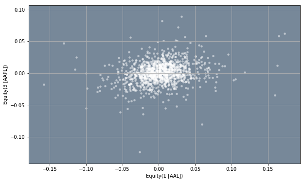
Correlation of Returns
Apart from visualizing the correlation between stocks as we did above, we can also create a correlation dataframe that gives the correlation between every stock. In the code below, we can accomplish this using the .corr() method to calculate the correlation between all the paris of stocks in our returns dataframe.
# Display the correlation between all stock pairs in the returns dataframe
returns.corr(method = 'pearson').head()| Equity(0 [A]) | Equity(1 [AAL]) | Equity(2 [AAP]) | Equity(3 [AAPL]) | Equity(4 [ABBV]) | Equity(5 [ABC]) | Equity(6 [ABT]) | Equity(7 [ACN]) | Equity(8 [ADBE]) | Equity(9 [ADI]) | ... | Equity(481 [XL]) | Equity(482 [XLNX]) | Equity(483 [XOM]) | Equity(484 [XRAY]) | Equity(485 [XRX]) | Equity(486 [XYL]) | Equity(487 [YUM]) | Equity(488 [ZBH]) | Equity(489 [ZION]) | Equity(490 [ZTS]) | |
|---|---|---|---|---|---|---|---|---|---|---|---|---|---|---|---|---|---|---|---|---|---|
| Equity(0 [A]) | 1.000000 | 0.327356 | 0.350274 | 0.357941 | 0.219881 | 0.443607 | 0.498730 | 0.528160 | 0.476105 | 0.488426 | ... | 0.547015 | 0.448453 | 0.520123 | 0.568743 | 0.524692 | 0.333886 | 0.405655 | 0.485227 | 0.524167 | 0.186108 |
| Equity(1 [AAL]) | 0.327356 | 1.000000 | 0.243475 | 0.227264 | 0.143983 | 0.296306 | 0.244604 | 0.269950 | 0.308133 | 0.285740 | ... | 0.361259 | 0.241502 | 0.177152 | 0.356118 | 0.258117 | 0.173434 | 0.254696 | 0.289684 | 0.344630 | 0.138426 |
| Equity(2 [AAP]) | 0.350274 | 0.243475 | 1.000000 | 0.210157 | 0.211495 | 0.290848 | 0.329866 | 0.293221 | 0.301972 | 0.309280 | ... | 0.312257 | 0.289204 | 0.282981 | 0.346646 | 0.275858 | 0.268899 | 0.329385 | 0.302148 | 0.329689 | 0.150945 |
| Equity(3 [AAPL]) | 0.357941 | 0.227264 | 0.210157 | 1.000000 | 0.124744 | 0.261941 | 0.260044 | 0.345766 | 0.317921 | 0.384693 | ... | 0.292361 | 0.284832 | 0.320862 | 0.342525 | 0.322910 | 0.251614 | 0.297765 | 0.333980 | 0.349393 | 0.155476 |
| Equity(4 [ABBV]) | 0.219881 | 0.143983 | 0.211495 | 0.124744 | 1.000000 | 0.265333 | 0.355565 | 0.214197 | 0.223873 | 0.256881 | ... | 0.163470 | 0.235468 | 0.229631 | 0.247383 | 0.226287 | 0.253060 | 0.203928 | 0.304504 | 0.183191 | 0.340621 |
5 rows × 490 columns
As we can see, this is a better way to see how correlated the stock returns are than through visulaization. By looking at the table we can easily spot which pairs of stock have the highest correlation.
TODO:
In the code below, make a scatter of equity A and equity XOM.
%matplotlib inline

import matplotlib.pyplot as plt

# Set the default figure size
plt.rcParams['figure.figsize'] = [10.0, 6.0]

# # Make scatter plot
ax = returns.plot.scatter(x = 0, y = 483, grid = True, color = 'white', alpha = 0.5, linewidth = 0)

ax.set_facecolor('lightslategray')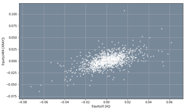
TODO:
In the code below, write a function get_num_components(df, var_ret) that takes a dataframe, df, and a value for the desired amount of variance you want to retain from the df dataframe,var_ret. In this case, the parameter df should be the returns dataframe obtained above. The parameter var_ret must be anumber between 0 and 1. The function should return the number of principal components you need to retain that amount of variance. To do this, use Scikit-Learn's PCA() class and its .explained_variance_ratio_. The function should also print the total amount of variance retained.
# import resources
from sklearn.decomposition import PCA

def get_num_components(df, var_ret):

    if var_ret > 1 or var_ret < 0:
        print('Error')
        return 0

    if var_ret == 1:
        return df.shape[1]

    pca = PCA(n_components = df.shape[1])

    pca.fit(df)

    needed_components = 0

    var_sum = 0

    for i in range(0, df.shape[1]):

        if var_sum >= var_ret:
            print('Total Variance Retained: ', pca.explained_variance_ratio_[0:needed_components].sum())
            return needed_components
        else:
            needed_components += 1
            var_sum += pca.explained_variance_ratio_[i]

num_components = get_num_components(returns, 0.9)

print('\nNumber of Principal Components Needed: ', num_components)
Total Variance Retained: 0.900236862496
Number of Principal Components Needed: 179TODO:
In the previous section you calculated the number of principal compenents needed to retain a given amount of variance. As you might notice you can greatly reduce the dimensions of the data even if you retain a high level of variance (var_ret > 0.9). In the code below, use the number of components needed calculated in the last section, num_components to calculate by the percentage of dimensionality reduction. For example, if the original data was 100-dimensional, and the amount of components needed to retian a certain amount of variance is 70, then we are able to reduce the data by 30%.
# Calculate the percentage of dimensionality reduction
red_per = ((returns.shape[1] - num_components) / returns.shape[1]) * 100

print('We were able to reduce the dimenionality of the data by:', red_per, 'percent')
We were able to reduce the dimenionality of the data by: 63.469387755102034 percentfunction helper
utils.py
import os

import pandas as pd

from zipline.data import bundles
from zipline.pipeline import Pipeline
from zipline.data.data_portal import DataPortal
from zipline.utils.calendars import get_calendar
from zipline.pipeline.data import USEquityPricing
from zipline.data.bundles.csvdir import csvdir_equities
from zipline.pipeline.factors import AverageDollarVolume
from zipline.pipeline.engine import SimplePipelineEngine
from zipline.pipeline.loaders import USEquityPricingLoader

# Specify the bundle name
bundle_name = 'm4-quiz-eod-quotemedia'

# Create an ingest function
ingest_func = csvdir_equities(['daily'], bundle_name)

# Register the data bundle and its ingest function
bundles.register(bundle_name, ingest_func);

# Set environment variable 'ZIPLINE_ROOT' to the path where the most recent data is located
os.environ['ZIPLINE_ROOT'] = os.path.join(os.getcwd(), '..', '..', 'data', 'module_4_quizzes_eod')

# Load the data bundle
bundle_data = bundles.load(bundle_name)

# Create a screen for our Pipeline
universe = AverageDollarVolume(window_length = 120).top(500)

# Create an empty Pipeline with the given screen
pipeline = Pipeline(screen = universe)

# Set the dataloader
pricing_loader = USEquityPricingLoader(bundle_data.equity_daily_bar_reader, bundle_data.adjustment_reader)

# Define the function for the get_loader parameter
def choose_loader(column):
    if column not in USEquityPricing.columns:
        raise Exception('Column not in USEquityPricing')
    return pricing_loader

# Set the trading calendar
trading_calendar = get_calendar('NYSE')

# Create a Pipeline engine
engine = SimplePipelineEngine(get_loader = choose_loader,
                              calendar = trading_calendar.all_sessions,
                              asset_finder = bundle_data.asset_finder)

# Set the start and end dates
start_date = pd.Timestamp('2016-01-05', tz = 'utc')
end_date = pd.Timestamp('2016-01-05', tz = 'utc')

# Run our pipeline for the given start and end dates
pipeline_output = engine.run_pipeline(pipeline, start_date, end_date)

# Get the values in index level 1 and save them to a list
universe_tickers = pipeline_output.index.get_level_values(1).values.tolist()

# Create a data portal
data_portal = DataPortal(bundle_data.asset_finder,
                         trading_calendar = trading_calendar,
                         first_trading_day = bundle_data.equity_daily_bar_reader.first_trading_day,
                         equity_daily_reader = bundle_data.equity_daily_bar_reader,
                         adjustment_reader = bundle_data.adjustment_reader)

def get_pricing(data_portal, trading_calendar, assets, start_d, end_d, field='close'):

    # Set the given start and end dates to Timestamps. The frequency string C is used to
    # indicate that a CustomBusinessDay DateOffset is used
    end_dt = pd.Timestamp(end_d, tz='UTC', freq='C')
    start_dt = pd.Timestamp(start_d, tz='UTC', freq='C')

    # Get the locations of the start and end dates
    end_loc = trading_calendar.closes.index.get_loc(end_dt)
    start_loc = trading_calendar.closes.index.get_loc(start_dt)

    # return the historical data for the given window
    return data_portal.get_history_window(assets=assets, end_dt=end_dt, bar_count=end_loc - start_loc,
                                          frequency='1d',
                                          field=field,
                                          data_frequency='daily')

def get_returns(start_date='2011-01-05', end_date='2016-01-05'):

    # Get the historical data for the given window
    historical_data = get_pricing(data_portal, trading_calendar, universe_tickers,
                                  start_d=start_date, end_d=end_date)

    return historical_data.pct_change()[1:].fillna(0)
为者常成,行者常至
自由转载-非商用-非衍生-保持署名(创意共享3.0许可证)


